Kalman Filter Learning Series
Part of the AI Hardware Engineer Roadmap.
Learning Path
| Level | Chapters |
|---|---|
| Start | 00 - Index |
| Elementary | 01 · 02 · 03 |
| Middle School | 04 · 05 · 06 |
| High School | 07 · 08 · 09 |
| Linear algebra and noise | 10 · 11 · 12 · 13 |
| Nonlinear estimation | 14 · 15 · 16 · 17 |
| Numerics and integration | 18 · 19 · 20 · 21 |
Reference
First reproducible experiment: Camera geometry and delayed sensor fusion on CPU. It includes a dependency lock, measured results, failure injections, and analytic tests. Use implementation templates to connect each lesson to code.
Example Outputs
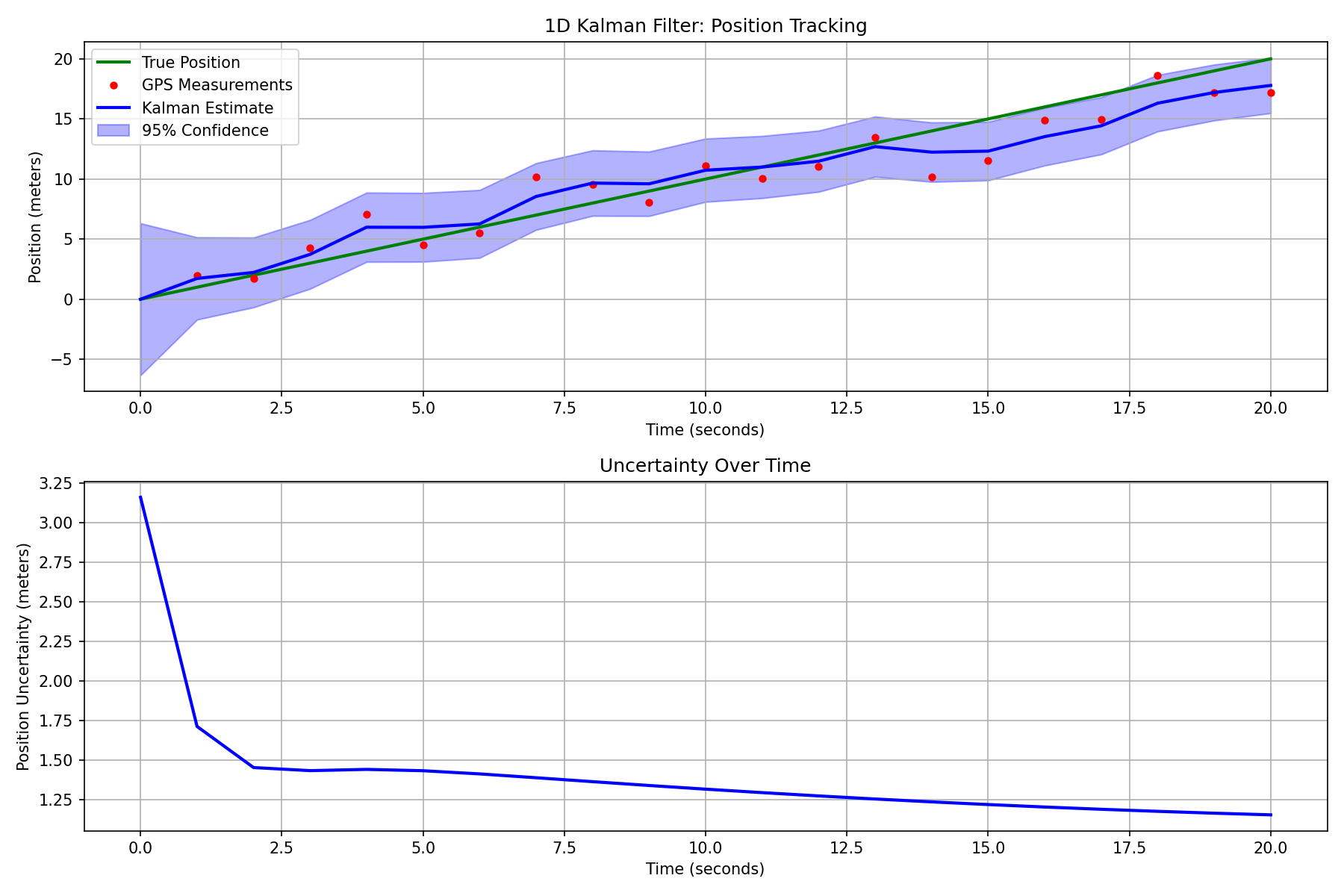
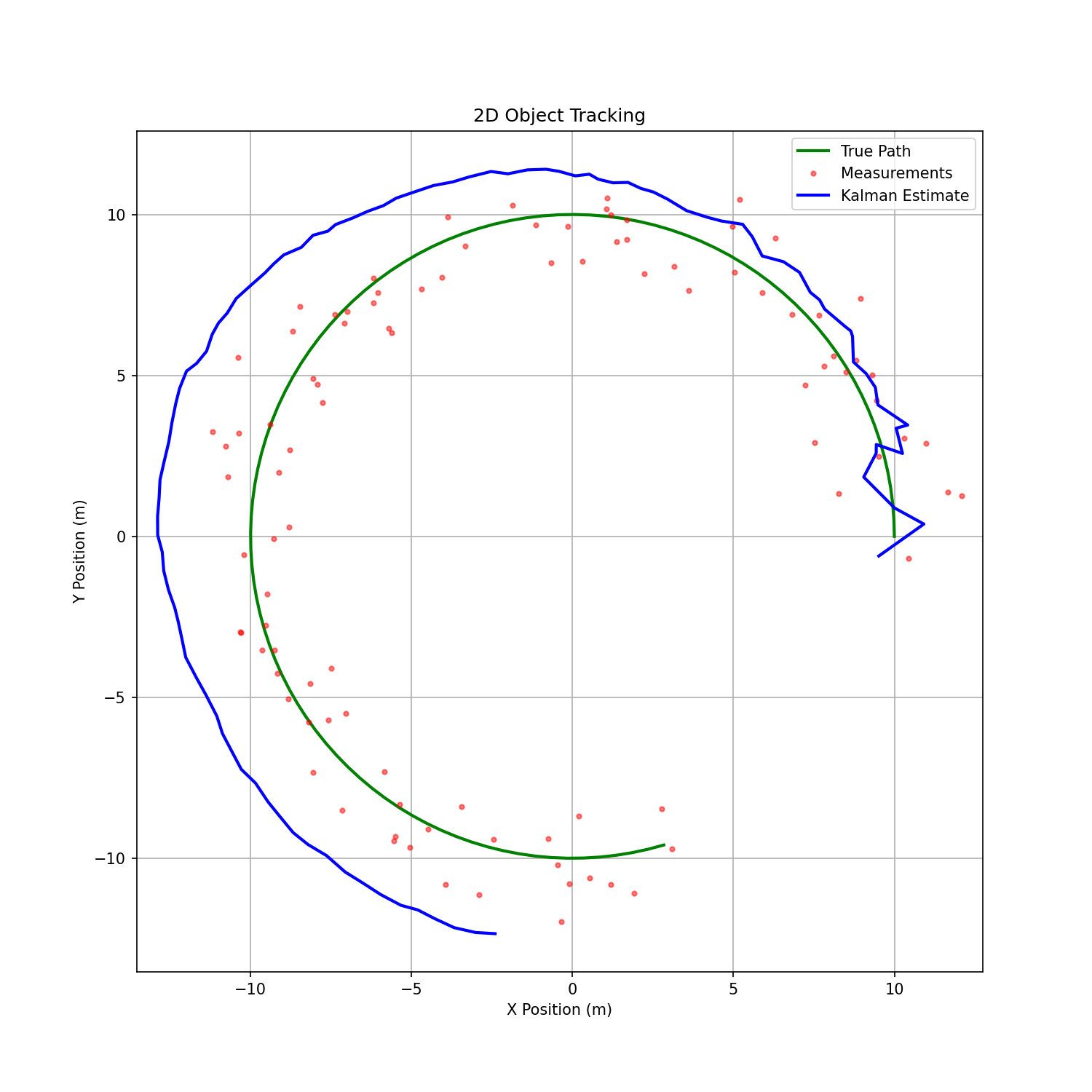
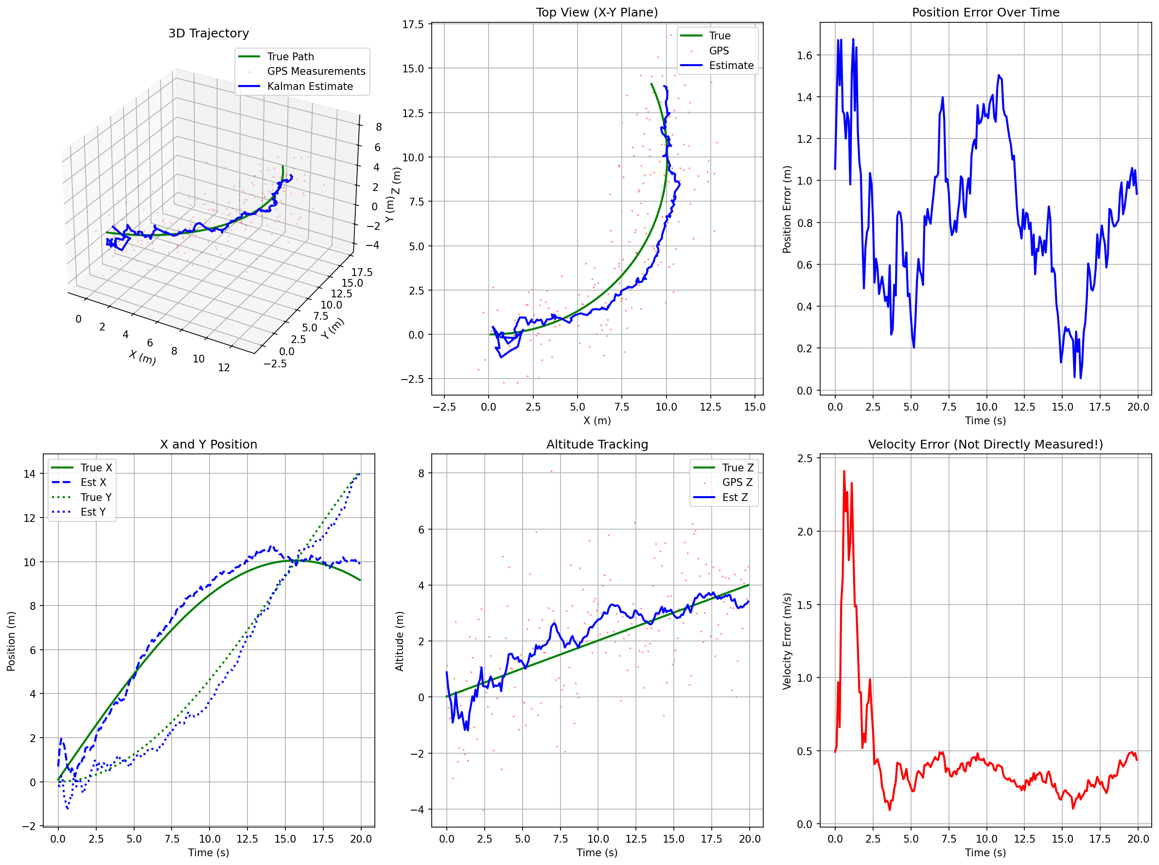
Run and check the original examples
From this directory, use an existing isolated NumPy environment or create a virtual environment for plotting:
python3 -m venv /tmp/kalman-course-venv
/tmp/kalman-course-venv/bin/python -m pip install numpy matplotlib
/tmp/kalman-course-venv/bin/python kalman_1d.py  # or kalman_2d.py, kalman_6d.py
/tmp/kalman-course-venv/bin/python -m unittest discover \
  -s ../Camera-Time-Fusion-Lab/labs/optional -p test_series_covariance.py -v
The eight numerical tests need NumPy only; importing the filter classes does not import Matplotlib or open a window. Plotting functions save images next to their scripts. The 2D circle uses exactly 0.1-second intervals and seed 42. A constant-velocity model deliberately mismatches curved motion, so its smooth output does not establish calibrated uncertainty.
Worked checks: reproduce the train update in lesson 07, then run the tests. They verify the entire covariance, flat/column measurement parity, rejection of row-vector broadcasting, defensive copies, invalid covariance/noise inputs, and 500 sequential 2D updates against the general filter. The scalar counterexample F=.5,P=16,Q=0 predicts variance 4; H=−.5,R=1 then gives gain −1. Thus prediction need not increase variance, and a general gain need not lie in [0,1].
The general example accepts x0 with shape (n,1) and observations (m,) or (m,1). It requires finite real inputs, symmetric positive-semidefinite P0/Q, and positive-definite R; it copies caller-owned arrays. These are this implementation's contracts, not a claim that every valid Kalman model needs strictly positive measurement noise. Missing observations mean predict only. For timestamps, gating, delayed replay and nonlinear extensions, continue to the camera/time lab.
Reviewed with NumPy 2.3.5 for the numerical suite; all three plots also executed headlessly with system NumPy 1.26.4 / Matplotlib 3.6.3 into a temporary directory. Recorded checks and source hashes. Matrix gain uses a linear solve, and correction uses Joseph form. See lesson 20 for the limits of numerical repairs.
External
Carry this course into the physical-AI system
Start from: A seeded trajectory and explicit process/measurement noise.
Build and challenge: Compare prediction-only, measurement-only, and filtered estimates. Double the sample interval and introduce dropout; inspect innovation and covariance as well as state error.
Pass forward: An estimator with documented time-step and uncertainty assumptions. Continue with the connected course and keep the artifact in the Physical AI Design Studio.