A systems field report on building a tensor-parallel inference engine for Qwen2.5-72B-Instruct on 8×H200. Spoiler: at TP=8 the bottleneck is almost never the matmul. It’s the barrier.
Table of contents
Open Table of contents
- 0. TL;DR
- What is the real bottleneck?
- 1. Why hand-build an engine when vLLM and SGLang exist?
- 2. The two-phase reality: prefill and decode are different machines
- 3. Profiling decode at TP=8: the all-reduce is the giant
- 4. The key finding: the all-reduce is barrier-bound, not bandwidth-bound
- 5. The TTFT problem: death by a thousand host syncs
- 6. The kernel work — including where it didn’t help
- 7. The correctness trap that TP makes uniquely nasty
- 8. Profiling when the profiler is taken away
- 9. The honest scorecard: TP=1 and TP=4 win, TP=8 doesn’t
- 10. The communication primitive: put-with-signal, no host in the loop
- 11. The meta-lessons (what I’d tell past-me)
- References
0. TL;DR
I built a custom tensor-parallel serving engine for Qwen2.5-72B (decoder-only) and spent most of the project staring at profiles. The single most valuable thing I learned: at tensor-parallel degree 8, you are not compute-bound and you are barely bandwidth-bound on the matmuls — you are bound by synchronization.
- Decode budget at TP=8: all-reduce ~50%, MLP ~28%, attention ~24%. The communication barrier is the single largest line item, larger than all the matrix multiplies combined.
- Prefill / TTFT: death by host syncs — 332
cudaStreamSynchronizeper request ≈ 56% of CPU time, producing a ~2× time-to-first-token gap vs a tuned baseline. - The actual matmul kernels were already near the roofline (~87% memory-bandwidth utilization on the decode GEMV). There was almost no headroom in the math.
- My most expensive mistakes were guessing instead of profiling, and trusting benchmarks from the wrong regime.
- The regime picks the winner: the engine beats vLLM at TP=1 (single GPU, +21% decode) and TP=4 (+1.7% → +3.76% end-to-end with FlashInfer attention + my custom communication, plus +25% decode via speculative decode), and ties at TP=2. The loss is specific to TP=8 — and the tell is scaling: vLLM’s decode climbs 44 → 92 tok/s from TP=2 to TP=8 while mine regresses 44 → 38, because the O(TP) barrier tax grows faster than the bandwidth gain (§9).
This is the engine-engineering companion to my work on multi-token prediction. That one was about generating more tokens per weight-read; this one is about the brutal truth of one weight-read across 8 GPUs. And to see the forward pass behind these numbers — each stage landing memory- or compute-bound on an H200 roofline, and the weights sharding (with the all-reduce cost growing) as you slice across TP = 1 / 2 / 4 / 8 — I built an interactive LLM Inference Visualizer.
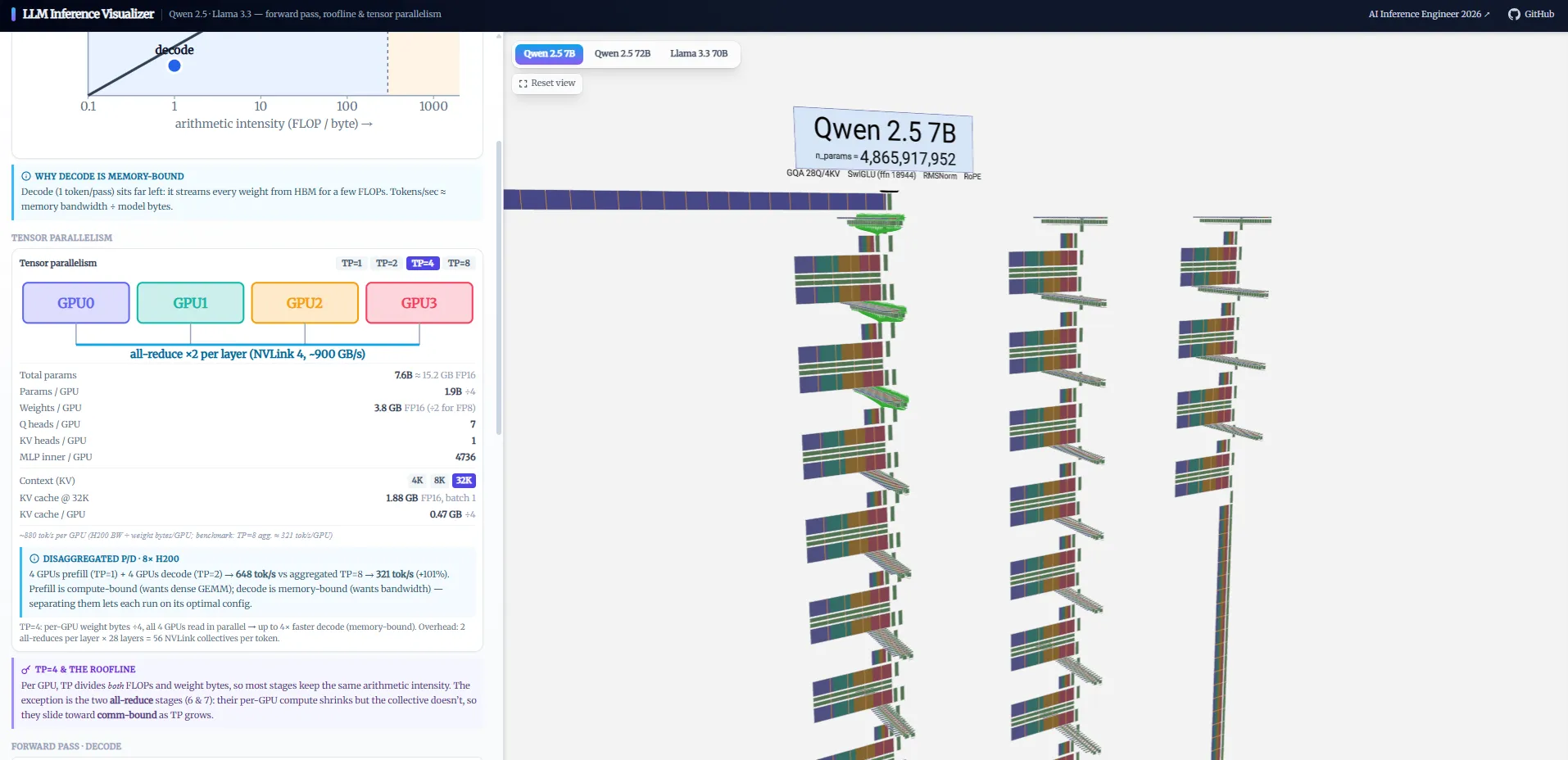
Click to open the visualizer live — walk the forward pass, the roofline, and TP sharding interactively.
What is the real bottleneck?
Before the sections: here is the answer, stated plainly, so nothing that follows is a surprise.
Prefill (TTFT) bottleneck: host synchronization, not compute. The tensor-core GEMMs in prefill are fast — they run near the roofline at high arithmetic intensity. The bottleneck is the host orchestrating each layer’s all-reduce: 332 cudaStreamSynchronize per request consume ~56% of CPU time and produce a ~2× TTFT gap vs a baseline that graph-captures the same work.
Decode bottleneck: the all-reduce barrier, not the matmuls and not the bandwidth. The decode GEMV already reaches ~87% of peak HBM bandwidth — the matmuls are essentially solved. The binding cost is the collective synchronization: at TP=8, each decoded token requires ~160 all-reduces, each costing ~6.9 µs, of which >99% is the barrier (making 8 GPUs agree they’ve all arrived) and <1% is data movement. NVLink 5.0 has 900 GB/s of bandwidth; the 16 KB all-reduce message could cross in 0.018 µs. The 6.9 µs is the handshake, not the pipe.
The corollary — why the engine anti-scales at TP=8. Decode is memory-bound: more GPUs → each reads fewer weight bytes per token → throughput should scale. It does for vLLM (44 → 92 tok/s, TP=2→8). For the engine (44 → 38 tok/s), the O(TP) barrier tax grows faster than the bandwidth gain, and adding GPUs makes decode slower. Amdahl’s law with 50% barrier fraction caps the TP=8 speedup at ~1.78× over TP=1 regardless of how fast the matmuls are.
The fix — in-kernel, host-free barriers + CUDA-graph capture. Everything that follows is an elaboration of that fix.
1. Why hand-build an engine when vLLM and SGLang exist?
You shouldn’t, for production. vLLM, SGLang, and TensorRT-LLM are superb and you will not beat them on a Tuesday. I built one anyway because building the engine is the only way to truly learn where the microseconds go. When you own the all-reduce, the attention kernel, and the CUDA-graph capture, the profiler stops being abstract and starts being a to-do list.
The target — Qwen2.5-72B-Instruct — is a good teacher: 80 decoder layers, grouped-query attention (far fewer KV heads than query heads), 8192 hidden, a ~152k vocab, sharded 8 ways across a single H200 node. Big enough that every inefficiency is visible; standard enough that the lessons transfer.
2. The two-phase reality: prefill and decode are different machines
The first conceptual unlock is that an autoregressive LLM serving loop is two completely different workloads wearing one model:
| Prefill (process the prompt) | Decode (generate each token) | |
|---|---|---|
| Batched over | all prompt tokens at once | 1 token (at batch size 1) |
| Bottleneck | compute (big GEMMs, tensor cores hot) | memory (stream all weights per token) |
| Scales with | sequence length × FLOPs | weight bytes / HBM bandwidth |
| Owns | time-to-first-token (TTFT) | inter-token latency / throughput |
They want opposite optimizations, and the #1 profiling mistake — which I made — is letting one contaminate the other’s profile (see §6.2). Always split them.
The H200 roofline in concrete numbers
Understanding why the bottleneck is where it is requires knowing the hardware budget. The NVIDIA H200 SXM:
| H200 SXM spec | Value |
|---|---|
| HBM3e bandwidth | 3.35 TB/s |
| BF16 tensor-core TFLOPS | ~989 TFLOPS |
| FP8 tensor-core TFLOPS | ~1,979 TFLOPS |
| NVLink 5.0 bandwidth (per GPU, bidirectional) | ~900 GB/s |
| Ridge point (BF16) | ~295 FLOPs/byte |
The decode roofline at TP=1. Qwen2.5-72B in BF16 is ~144 GB of weights. At batch=1 decode, every generated token streams the entire model from HBM:
Theoretical decode ceiling (TP=1, BF16):
  144 GB ÷ 3.35 TB/s ≈ 43 ms/token → ~23 tok/s
That is the physics ceiling for a single H200 before any kernel overhead, KV reads, or synchronization.
The TP=8 bandwidth ceiling. Eight H200s each hold 18 GB (144/8) of weights. With a perfect all-reduce (zero cost), eight GPUs contribute a proportional speedup:
Theoretical decode ceiling (TP=8, BF16, perfect comms):
  18 GB ÷ 3.35 TB/s ≈ 5.4 ms/token → ~185 tok/s
vLLM achieves 92 tok/s (50% of theoretical). The custom engine in its default state achieved 10 tok/s (5.4% of theoretical), rising to 38 tok/s (21%) after the custom communication fast path (§10). The 79% gap between theory and practice lives entirely in the all-reduce synchronization. This is not a rounding error — it is the dominant term in the budget.
Why prefill is compute-bound, not bandwidth-bound. At prefill with an N-token prompt, the weight matrices are read once but the activations are N×. The arithmetic intensity of a (B=N, K, M) GEMM is 2×N×K×M / (K×M bytes) = 2×N — it scales with prompt length. For N=512 tokens (a medium prompt), intensity = 1024 FLOPs/byte, which is well above the H200 BF16 ridge point of 295 FLOPs/byte. Tensor cores are the bottleneck. For N=1 (decode), intensity = 2 FLOPs/byte — 150× below the ridge point. Pure memory bottleneck. The same model, the same GPU, two completely different constraints.
3. Profiling decode at TP=8: the all-reduce is the giant
Here is the decode-step breakdown that reorganized my whole mental model (TP=8, per-token, steady state):
The all-reduce dominates. Not the 72-billion-parameter matrix multiplies — the communication. Once you see it, the reason is obvious. Tensor parallelism splits every weight matrix across the 8 GPUs, so after the attention block and after the MLP block of every one of the 80 layers, the partial results must be summed across all 8 ranks. That’s ~160 all-reduces per generated token.
And here’s the cruel part: at decode (batch 1), each all-reduce moves a tiny tensor — a single token’s hidden vector:
hidden_size = 8192 dimensions × 2 bytes (BF16) = 16 KB per all-reduce message
160 all-reduces/token × 16 KB = 2.56 MB total data movement per token
At NVLink 5.0’s 900 GB/s per-GPU bidirectional bandwidth, that 16 KB message could theoretically transit in ~0.018 µs. The measured cost is ~6.9 µs per all-reduce — making the actual data movement <0.3% of the cost. What costs you is making 8 GPUs agree they’ve all arrived — the barrier — 160 times per token, on the critical path of a memory-bound loop where the GPU is otherwise idle waiting on HBM anyway.
160 all-reduces × 6.9 µs = ~1.1 ms per token in bare synchronization overhead, on top of the weight-read time. At a theoretical 185 tok/s ceiling that’s already burning 20% of the per-token budget on barriers before you write a single kernel line.
4. The key finding: the all-reduce is barrier-bound, not bandwidth-bound
This is the insight I’m proudest of, because I almost optimized the wrong thing.
The intuitive fix for “all-reduce is slow” is to move the data faster — and NVLink offers multimem (hardware multicast) exactly for that. I spent real effort getting multimem correct (multicast supported, bit-exact) and then benchmarked it head-to-head against a plain peer-to-peer one-shot in-kernel reduce:
16 KB message, 4-way:
   multimem (multicast)        6.92 µs
   peer-N one-shot in-kernel   6.93 µs     ← identical
Identical. The data-movement optimization bought nothing, because at this size the data movement is <1% of the 6.9 µs. The entire cost is the barrier — the round of synchronization. So the lever isn’t a faster pipe; it’s a cheaper handshake.
That reframes the all-reduce engineering completely:
- The naive way (what I started with): a host-orchestrated barrier — each rank signals an event, the host waits on all of them, then launches the reduce. That’s a CPU↔GPU round-trip per all-reduce, ×160 per token. Murder.
- What the good engines do: an in-kernel flag barrier — a single fused kernel where each rank writes a flag to peer memory and spins until it sees all peers’ flags, then reduces, with no host in the loop. vLLM ships exactly this kind of hand-written single-node all-reduce kernel (with an NCCL fallback), and it’s why it’s fast at TP=8.
- The frontier (where I aimed): TensorRT-LLM’s Lamport-style, barrier-free one-shot — rank k spins directly on the data arriving (using a sentinel value like
-0.0to distinguish “written” from “not yet”), so there is no separate barrier at all, triple-buffered to stay correct across iterations and CUDA-graph-capturable. Because my engine was single-process (one rank per GPU thread in one process, no IPC), this was actually simpler to implement than the multi-process reference designs.
Lesson: when a collective is small-message-dominated, profile the barrier, not the bandwidth. Multicast, fancier reduction trees, and bigger NVLink all optimize the part that wasn’t the problem.
5. The TTFT problem: death by a thousand host syncs
While decode was within a few percent of the reference, TTFT was ~2× worse. The profiler handed me the murder weapon immediately:
332 cudaStreamSynchronize per request ≈ 56% of total CPU timeThe cause: my prefill was running eager (not CUDA-graph-captured, because prompt lengths vary), and every layer’s all-reduce was followed by a sync_all() — a host round-trip to make sure the collective finished before proceeding. O(TP) host syncs × 80 layers × (attn + mlp) = hundreds of cudaStreamSynchronize calls per request, each one stalling the CPU while the GPU idles. The decode path didn’t have this problem because it was graph-captured — the whole step replays on the GPU with no per-step host involvement.
The fix is three independent levers, all aimed at getting the host out of the loop:
- In-kernel prefill all-reduce — the barrier-free barrier from §4, so no
sync_allis needed. - Bucketed prefill graphs — you can’t graph arbitrary prompt lengths, but you can capture a handful of length buckets and pad into them, recovering graph replay for prefill.
- On-device argmax — don’t copy the logits back to the host to pick the next token; do the argmax on the GPU. One fewer host sync on the hottest path.
A first cut (a two-shot prefill all-reduce that removed one host sync per layer) already shaved TTFT a consistent ~1.3% with no quality change — small, but it confirmed the model: TTFT was a host-sync problem, not a compute problem.
6. The kernel work — including where it didn’t help
6.1 Decode GEMV: already near the roofline
The decode matmuls are tall-skinny GEMVs (matrix × single-token vector), pure memory-bound. I wrote a row-tiled GEMV with vectorized FP8 dequant and measured it against the roofline using MBU (Memory Bandwidth Utilization = achieved bytes/s ÷ peak HBM bytes/s):
- Row-tiling lifted decode from ~50.8 → ~54.7 tok/s (at TP=2) and hit ~87% MBU on the bf16
down_proj.
87% of peak HBM bandwidth means there’s ~13% left on the table, total. The GEMV was essentially solved; chasing it further was diminishing returns. This is the FlashInfer lesson generalized — decode is IO-bound and a good kernel runs close to the bandwidth ceiling; once you’re there, the math is done and the remaining time is elsewhere (the barrier, §4).
6.2 The cuBLASLt ghost (a profiling cautionary tale)
For a while I “knew” decode had a 12.6% activation-quantization overhead in its cuBLASLt path, and I planned a kernel to remove it. Then I split the profile properly and found the truth: that 12.6% was prefill contamination leaking into the decode bucket. Decode already used a weight-only FP8 GEMV — it never quantized the activation at all. The overhead I was about to spend a week deleting did not exist at decode. I had been about to optimize a ghost. Lesson: if your prefill and decode share a profiling bucket, you will chase phantoms. Separate them before you believe any number.
6.3 Custom decode attention: parity at TP=8, regression at TP=4
I wrote a GQA-aware, warp-level flash-decoding attention kernel tuned for Qwen2.5-72B on Hopper. GQA is the right place to optimize because its low KV-head count raises arithmetic intensity (FlashInfer makes the same observation and even runs a prefill-style Tensor-Core kernel for GQA decode). Results:
- TP=8: ~74.7 tok/s, parity with FlashInfer, output bit-identical. A real, owned kernel matching the best available.
- TP=4: custom 58.2 vs FlashInfer 67.9 — my kernel was 14% slower.
The custom kernel’s fixed 256-way split grid was tuned for TP=8’s small per-GPU KV slice; at TP=4, each GPU holds twice the KV and that grid was over-provisioned, wasting occupancy. Same kernel, two TP degrees, opposite verdict. I kept FlashInfer as the default and would only deploy the custom kernel in the exact regime it won. (This regime-dependence theme runs through everything in TP land.)
7. The correctness trap that TP makes uniquely nasty
I “improved” my in-kernel barrier flag from a toggle (!= flag) to a monotonically-increasing counter (< flag). It benchmarked +3% at TP=4 and passed a 5,000-iteration A/B. Shipped.
Then, over a full run across all 8 ranks and many prompts, decode throughput snowballed downward: 86 → 35 tok/s over 9 prompts. The monotonic flag let the 8 ranks desync progressively — a tiny drift each step that compounded across ranks and time until the barrier was effectively serializing everything. The toggle version was self-correcting; the “optimized” counter version was not. I reverted.
Lesson: tensor-parallel correctness bugs hide in the interaction of many ranks over many steps. A short, single-prompt, low-rank A/B test is exactly the test that won’t catch them. If a TP optimization isn’t validated over a long multi-prompt run at the deployment rank count, you haven’t validated it.
8. Profiling when the profiler is taken away
A practical note: on the rented multi-GPU nodes, ncu and nsys were blocked (CUPTI returned “no kernel data” — common on locked-down/cloud instances). You can still profile: I built a CUDA-event timing harness — wrap each stage (qkv, attn, o_proj, mlp, all_reduce, lm_head) in cudaEventRecord pairs and accumulate per-stage microseconds, plus counters for things like cudaStreamSynchronize calls. Every profile number in this post came from that in-process instrumentation, not from a vendor profiler. You don’t need ncu to find your bottleneck; you need to instrument your own code.
9. The honest scorecard: TP=1 and TP=4 win, TP=8 doesn’t
The same engine gives different verdicts at different tensor-parallel degrees — it beats vLLM at TP=1 and TP=4, ties at TP=2, and loses at TP=8 — and that split is the headline result.
At TP=4 the engine beats vLLM. Running FlashInfer’s attention (my custom kernel loses at TP=4 — §6.3) on top of my custom in-kernel communication, it comes in +1.7% to +3.76% ahead of vLLM end-to-end, with TTFT at parity (~303 ms). Layer speculative decode on top and decode throughput reaches ~85 tok/s vs vLLM’s ~68 — a +25% decode win.
At TP=8 the same code loses (~−11% end-to-end), and almost all of the gap is TTFT (~409 ms vs ~200 ms — ~2× slower) — the host-sync problem from §5. Decode is the other half of the story. With speculative decode, throughput is near-parity (~86 vs ~89 tok/s, −4%) — but that masks how far behind the base decode is. Without spec, raw decode is ~38 vs ~92 tok/s (0.42×), and that is after the custom-comm fast path from §10 (peer one-shot all-reduce + joint decode graphs) already lifted it 3.7×, from ~10 to ~38. The custom communication is doing real work; at 8 ranks it just isn’t enough yet.
| TP=4 (H200) | TP=8 (H200) | |
|---|---|---|
| End-to-end vs vLLM | +1.7% → +3.76% — win | ~−11% — loss |
| TTFT | ~303 ms (≈ parity) | ~409 ms vs ~200 ms (~2×) |
| Decode TPS | ~85 vs ~68 with spec (+25%) | ~86 vs ~89 with spec (−4%); ~38 vs ~92 base |
| Decode GEMV | ~87% MBU (near roofline) | ~87% MBU |
| Decode attention | FlashInfer (custom kernel loses here) | custom kernel = FlashInfer parity |
The low end of the curve. At TP=1 — one GPU, where only the smaller Qwen2.5-7B fits (the 72B doesn’t) — there are no ranks to synchronize, the barrier tax is zero, and the engine wins clean: TTFT 17.7 ms vs 19.4 ms and 194 vs 160 tok/s decode (+21%). At TP=2 (the 72B on 2×H200) it’s a dead heat — decode throughput dead even (44.4 vs 44.0 tok/s), TTFT trailing slightly (561 vs 505 ms). Parity, no more.
The most telling number, though, isn’t any single verdict — it’s the slope. Watch raw decode throughput as the rank count climbs:
vLLM scales from TP=2 to TP=8 (44 → 92 tok/s); my engine regresses (44 → 38). That is the whole thesis in one line. Decode is memory-bound — it’s a weight read — so adding GPUs should help: more ranks shard the 72B further, each reads fewer bytes per token, throughput rises. It does, for vLLM. For my engine the O(TP) all-reduce barrier tax grows faster than the bandwidth gain, so more GPUs make decode slower. The custom-comm fast path from §10 bends the curve up hard — 3.7×, from 10 to 38 tok/s at TP=8 — but it’s bending a curve that still points the wrong way. Barrier-bound anti-scales; bandwidth-bound scales. Beating vLLM at TP=8 means making the engine bandwidth-bound again.
Amdahl’s law on the barrier. The anti-scaling has a clean analytical form. Suppose one decode step costs T_total = T_compute + T_barrier(TP). The compute term shrinks with TP (more GPUs, each reads fewer weights). The barrier term grows with TP (more ranks to synchronize). At TP=8 with a host-loop all-reduce, T_barrier ≈ 160 × 6.9 µs = 1.1 ms. If T_compute at TP=8 is ~7 ms (18 GB ÷ 3.35 TB/s × overhead), then barriers are already ~14% of the step — and with a slow host-loop implementation, they consume far more. Amdahl’s law says: if the non-parallelizable fraction is f, the speedup from P processors is bounded by 1/(f + (1-f)/P). With f = 0.5 (barriers = 50% of decode as measured), the TP=8 ceiling is 1/(0.5 + 0.5/8) = 1.78× over TP=1 — not 8×. The engine hits ~38 tok/s at TP=8, which is roughly TP=2 throughput (44 tok/s). The barrier tax is so large it makes adding GPUs destructive.
The honest read: one engine, one mechanism — the host-sync barrier cost is O(TP). At 1 rank there’s no barrier at all, so the engine wins outright; at 2 ranks the tax is small and it’s a tie; at 4 ranks it’s still tolerable and TTFT holds parity, so the near-roofline kernels and the custom communication carry the engine ahead; at 8 ranks the tax dominates, the 332 cudaStreamSynchronize land, TTFT goes 2×, and decode stops scaling. The frameworks’ edge at TP=8 isn’t exotic math — it’s in-kernel collectives and aggressive graph capture, i.e. synchronization engineering, and it only turns decisive as the rank count (and the barrier tax) grows.
10. The communication primitive: put-with-signal, no host in the loop
§4 and §5 both pointed at the same villain — the host round-trip — and the fix that runs through the whole engine is one idea: make the buffer I write into the doorbell I ring. The data channel and the synchronization channel become the same object. The producer never calls “send”; it writes activations straight into peer-visible memory and flips a signal word in the same slot, and the consumer was already watching that word. This is one-sided put-with-signal — the shape NVSHMEM exposes as nvshmemx_putmem_signal — except hand-rolled for a single process: no SHMEM runtime, no NCCL communicator, no proxy thread, and the whole handshake captured inside one CUDA graph.
cuStreamWaitValue32 on that word — zero SMs, captured as a single graph node, no host and no NCCL in the loop. Triple-buffering keeps a clean slot to write into when producer and consumer drift apart.The signal is a sentinel, not a spin. The lazy way to wait is an in-kernel spin — while (*flag == NOT_READY); — but that pins a resident warp and is opaque to graph capture. I gate the consumer’s stream with cuStreamWaitValue32 instead, which the stream front-end services in hardware: zero SMs, and it captures as a single graph node the executor can schedule around. The clever part is the sentinel. Each slot’s signal word is pre-armed to the bit pattern of -0.0f (0x80000000) — IEEE-754 negative zero, distinct from +0.0f (0x00000000) but a value real data never carries:
// proceed once the signal word's magnitude bits are nonzero —
// i.e. the slot no longer holds the ±0.0 sentinel
cuStreamWaitValue32(consumer_stream, signal, 0x7FFFFFFFu,
                    CU_STREAM_WAIT_VALUE_AND | CU_STREAM_WAIT_VALUE_FLUSH);
cuStreamWaitValue32 has exactly four compare modes — GEQ, EQ, AND, NOR — and each proceeds when its predicate is true, so there is no literal “wait until not-equal.” AND with 0x7FFFFFFF lands it: (*p & 0x7FFFFFFF) != 0 is false for both +0.0 and -0.0 (zero magnitude) and flips true the instant the producer’s token arrives. Keying off magnitude makes the slot self-arming — next iteration’s data overwrites the sentinel on its own, so a replayed decode graph needs no reset node. The one discipline: the anchor is a dedicated header word I own (pre-set to 0x80000000, written to a known nonzero token), never a live activation that could legitimately be 0.0 and stall the wait forever.
Ordering is the part that bites. A signal the consumer sees before the payload it guards is a silent corruption. Two valid shapes, never both: the producing kernel issues a system-scope __threadfence_system() before the release-store of the signal — system, not device, because it has to cross the link — or you let the kernel finish and signal with a cuStreamWriteValue32 node, whose default carries the barrier. And CU_STREAM_WAIT_VALUE_FLUSH on the waiter is what forces the peer’s outstanding writes to land before the poll reads them. (The volatile / ld.acquire advice you’ll read elsewhere applies only to a hand-rolled kernel spin — the thing we just deleted.)
Triple-buffering, because two races. With two slots, the moment the producer outruns the consumer — and it will, the instant an MoE expert imbalances or the KV cache grows — it laps and overwrites the slot being read. Not a deadlock; a torn read. Three slots decouple the timing with no sequence numbers and no backpressure: there’s always a clean slot to write into while one is in flight and one is being consumed. Three header words, rotated.
NVLink vs PCIe — probe, don’t hardcode. Remote WaitValue32 polling a peer’s signal is cheap over NVLink and a read-storm across a PCIe switch. So the primitive is chosen per peer-pair at startup:
cudaDeviceCanAccessPeer(&can, dev, peer);
cudaDeviceGetP2PAttribute(&atomics, cudaDevP2PAttrNativeAtomicSupported, dev, peer);
cudaDeviceGetP2PAttribute(&rank,    cudaDevP2PAttrPerformanceRank,       dev, peer);
PerformanceRank separates NVLink-class from PCIe-class links (NVML’s nvmlDeviceGetNvLinkState gives the explicit answer). NVLink with native remote atomics → wait directly on the peer slot. PCIe → flip to a writes-only shape: the consumer waits on a local word; the producer pushes payload, fences, then writes that local flag — so bus traffic is one-directional and nothing ever polls the narrow link.
Where this wins — and where it doesn’t. Put-with-signal is the right tool for everything that’s genuinely “my slice is ready”: pipeline-parallel stage handoffs, MoE expert routing, KV-cache ownership transfer, and the draft→target handoff in speculative decode (gate the verify kernel on the draft’s signal and the whole speculate→verify→continue loop never leaves the device). For all of those it beats ncclSend/ncclRecv on latency because there is nothing to launch. What it does not solve is the N-way collective — the all-reduce of §3 and §4, where eight ranks must agree they’ve all arrived. That barrier lives inside the fused reduce kernel (the SMs are busy reducing anyway, so the spin there isn’t wasted), and shipping its fully graph-captured form is the work between “beats vLLM at TP≤4” and “beats it everywhere.” Point-to-point is solved; the collective is the frontier.
11. The meta-lessons (what I’d tell past-me)
- Profile before you optimize. My two biggest time sinks — the cuBLASLt “ghost” and multimem — were both things the profiler would have told me not to bother with. Measure, then cut.
- At TP=8, the barrier is the workload. ~50% of decode is all-reduce, and that all-reduce is dominated by synchronization, not data movement. Invest in in-kernel, host-free barriers and CUDA-graph capture; deprioritize multicast and fancy reduction trees.
- Prefill and decode are different machines — different bottlenecks, different fixes, and they will poison each other’s profiles if you let them share a bucket.
- Regime-dependence is the law, not the exception. A kernel or flag that wins at TP=4 can lose at TP=8 (and vice versa); a number from H100 may not hold on H200. Validate only in the exact deployment regime — GPU, TP degree, and quantization all matter.
- TP correctness compounds over ranks × steps. Short A/B tests pass while long multi-rank runs rot. Validate at full scale, over many prompts.
- You can always profile. No
ncu? Instrument with CUDA events. The bottleneck is findable from inside your own process.
The headline, one more time: I went in expecting to win on kernels and lost on handshakes. A modern 72B serving engine on 8 GPUs is, more than anything, a distributed-systems synchronization problem wearing a deep-learning hat.
References
- vLLM — high-throughput LLM inference and serving engine (custom single-node all-reduce + NCCL fallback)
- vLLM — Parallelism and Scaling docs
- MSCCL++: Rethinking GPU Communication Abstractions for AI Inference — arXiv:2504.09014
- CUDA Driver API — Stream Memory Operations (
cuStreamWaitValue32/cuStreamWriteValue32) - NVSHMEM — signaling operations (one-sided put-with-signal)
- FlashInfer: Efficient and Customizable Attention Engine for LLM Inference — arXiv:2501.01005
- Accelerating Self-Attentions for LLM Serving with FlashInfer (decode attention is IO-bound; GQA optimization)
- Dissecting FlashInfer — A Systems Perspective on High-Performance LLM Inference
All profile numbers are from first-hand instrumentation of a single-node 8×H200 deployment of Qwen2.5-72B; treat them as one practitioner’s measurements, not a controlled study.