If you only internalize one mental model for LLM inference performance, make it the roofline. It explains, from two numbers on a datasheet, why decode is slow, why batching works, why quantization helps more than you’d expect, and why your tensor cores sit idle while you serve a single user.
Table of contents
Open Table of contents
Two numbers and one ratio
Every GPU has two peak rates that matter here:
- Compute — peak FLOP/s. For an H100 SXM5, the FP16 tensor cores do 989 TFLOPS (dense).
- Memory bandwidth — how fast it moves bytes from HBM. The H100 SXM5 has HBM3 at 3.35 TB/s.
A kernel is compute-bound if it’s limited by the first and memory-bound if limited by the second. Which one you hit depends on a property of the workload, not the hardware: arithmetic intensity (AI) — FLOPs performed per byte moved from memory.
arithmetic intensity = FLOPs / bytes moved [FLOP/byte]The crossover — the ridge point — is where the two roofs meet:
ridge point = peak FLOP/s / peak bytes/sFor the H100:
PEAK_FLOPS = 989e12      # FLOP/s   (FP16 tensor core, dense)
PEAK_BW    = 3.35e12     # bytes/s  (HBM3)

ridge_point = PEAK_FLOPS / PEAK_BW
print(f"{ridge_point:.0f} FLOP/byte")   # -> 295
295 FLOP/byte. A kernel must do ~295 FLOPs for every byte it reads from HBM just to keep the tensor cores busy. Below that, you’re starved on bandwidth and the compute units idle. (For an A100 the ridge sits around 153 FLOP/byte — lower peak compute, lower bandwidth, same story.)
The attainable throughput is the roofline itself:
def attainable_tflops(ai):
    """min(compute roof, bandwidth roof) at a given arithmetic intensity."""
    return min(PEAK_FLOPS, PEAK_BW * ai) / 1e12

attainable_tflops(1)     # ->   3.35 TFLOPS   (~0.3% of peak)
attainable_tflops(295)   # -> 989    TFLOPS   (right at the ridge)
attainable_tflops(600) # -> 989 TFLOPS (compute-bound, flat)Where decode lands
Autoregressive decode generates one token at a time. The dominant op is a matrix–vector product: every weight matrix W of shape [d_out × d_in] multiplies a single activation vector x.
Count it in FP16 (2 bytes/element), at batch size 1:
weights read : 2 · d_out · d_in   bytes      (each weight loaded once)
FLOPs        : 2 · d_out · d_in   FLOP        (one multiply + one add per weight)

AI = (2 · d_out · d_in) / (2 · d_out · d_in) = 1 FLOP/byte
One. Against a ridge point of 295. Single-stream decode runs at roughly 1/295 ≈ 0.3% of the H100’s tensor-core throughput. The expensive silicon NVIDIA built is almost entirely idle, because you spend all your time hauling weights across the memory bus to use each one exactly twice.
That single fact has a direct, quantitative consequence. If decode is bandwidth-bound, its speed is just bytes to move ÷ bandwidth. For a model with P parameters in FP16, you stream ~2P bytes per token:
params       = 8e9     # an 8B model
weight_bytes = 2 * params               # FP16 -> 16 GB / token

sol = weight_bytes / PEAK_BW            # speed-of-light latency
print(f"{sol*1e3:.2f} ms/token -> {1/sol:.0f} tok/s")
# 4.78 ms/token -> 209 tok/s   (upper bound, batch 1)
~209 tokens/s is the speed of light for an 8B model on one H100: you cannot decode faster without moving fewer bytes. Real numbers come in lower — attention reads the growing KV cache, not every op is on the tensor cores, kernel launches cost time, and you realistically sustain ~70–80% of peak HBM bandwidth. But the ceiling is set by bandwidth, full stop.
Why prefill is the opposite
Prefill — processing the T-token prompt before the first output token — does the same weight matrices against T activations at once. Weights are still read once; the FLOPs scale with T:
AI ≈ T (sequence length)A 512-token prompt gives AI ≈ 512 > 295 → compute-bound. So a single model runs in two completely different regimes:
| Phase | Op type | Arithmetic intensity | Bound by |
|---|---|---|---|
| Prefill | matrix–matrix | ≈ sequence length | Compute |
| Decode | matrix–vector | ≈ batch size | Bandwidth |
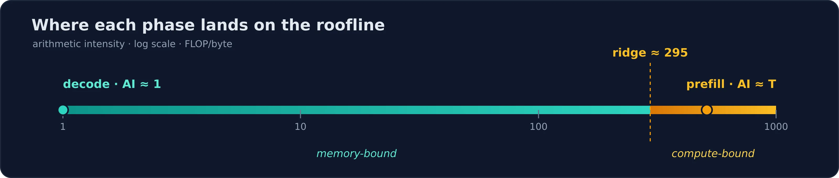
The same split as a number line: prefill’s intensity grows with sequence length T, clearing the ridge; batch-1 decode is pinned to the far left. Batching decode slides it rightward — AI ≈ batch size.
This is the reason prefill and decode get profiled, batched, and increasingly even scheduled on separate hardware — they stress opposite roofs.
Every decode optimization is a roofline move
Once you see decode pinned to the bandwidth roof at AI ≈ 1, the entire optimization playbook falls out of one question: how do I raise arithmetic intensity, or move fewer bytes?
- Batching raises AI directly. Decode
Bsequences together and they share one weight load: AI ≈B. To reach the ridge you needB ≈ 295— which is exactly why inference servers fight so hard to fill batches. (Continuous batching, e.g. vLLM, exists to keepBhigh without making users wait.) - Quantization cuts the bytes. INT8 weights halve the weight traffic vs. FP16; 4-bit roughly quarters it. Since you’re bandwidth-bound, ~half the bytes ≈ ~2× the tokens/s — the speedup tracks the byte reduction, not the FLOP reduction.
- KV-cache compression (MQA/GQA, paged or quantized KV) attacks the other growing source of bytes: attention re-reads the entire cache every step, and at long context it rivals the weights.
- Kernel fusion removes round-trips to HBM for intermediate activations — fewer bytes moved per useful FLOP, i.e. higher effective AI.
- FlashAttention is the same idea applied to attention: keep the
S = QKᵀscores in SRAM and never materialize the full[seq × seq]matrix in HBM. It’s a roofline win, not a FLOP win.
None of these are tricks. They’re all the same move — shift the workload rightward toward the ridge, or shrink the bytes under the bandwidth roof.
The takeaway
Before touching a profiler, you can predict the regime from a datasheet:
- Compute the ridge point:
peak FLOP/s ÷ peak bandwidth(~295 for an H100). - Estimate your kernel’s arithmetic intensity.
- If AI < ridge, you’re bandwidth-bound — chasing FLOPs is wasted effort; move fewer bytes or raise AI. If AI > ridge, optimize the compute.
Decode lives far to the left of the ridge, and almost everything we do to make inference fast is a structured campaign to drag it rightward. In the next posts I’ll measure a real decode kernel against this ceiling with Nsight Compute and see how much of the 0.3% → 100% gap is recoverable, and how much is physics.
Numbers cited are vendor peak specs for the H100 SXM5 (989 TFLOPS FP16 dense tensor; 3.35 TB/s HBM3). Peak ≠ achievable — I’ll always say which one I’m quoting.